Finding the Best Spot for a New Shop, One 50-Meter Square at a Time
A step-by-step spatial analysis of Sonadanga, Khulna — built with Python, GeoPandas, and open street map data, instead of a traditional desktop GIS tool.
Abstract
Where should a new shop or a new school go? People used to answer this question by walking around a neighborhood and guessing. This project answers it with data instead. I split a real neighborhood into thousands of small 50-meter squares, and gave every square a score based on three simple things: how close it is to a road, how close it is to homes, and how far it is from other shops. Then I combined the three scores into one final map that shows, in plain colors, exactly where the best spots are.
Why This Project Exists
Imagine you want to open a small shop. You have three questions in your head: Is it easy for people to reach? Do enough people live nearby to become customers? And is it far enough from other shops that already sell the same thing?
Normally, someone would answer these questions by feeling and experience. In this project, I answered them with numbers. I picked a real area — Sonadanga in Khulna city — and built a small computer program that looks at the whole area, square by square, and scores every square out of 1. A square with a high score is a great place for a new shop. A square with a low score is not.
This is called Site Suitability Analysis, and the method behind it is called Multi-Criteria Decision Analysis (MCDA) — a fancy name for a simple idea: take a few important factors, weigh them by how much they matter, and add them together.
Step One — Cutting the Map into Small Squares
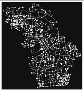
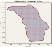
Most older suitability studies use raster grids — think of them like a photograph made of big, blocky pixels. Instead, I used a cleaner, more precise method: I drew the study area boundary of Sonadanga, and then covered it completely with small squares, each one 50 meters wide. Every square becomes its own independent unit that gets studied and scored on its own.
Why 50 meters? Because it is small enough to notice real differences between one street corner and the next, but not so small that the computer has to process millions of tiny fragments.
Step Two — Deciding What Matters, and How Much
Three factors decide whether a square is a good business spot. Each one gets turned into a score between 0 and 1, so that very different things — meters of distance, number of roads, number of shops — can all be compared fairly on the same scale.
Roads get the biggest weight because a shop nobody can reach is not a shop at all. Homes come next, since more nearby residents usually means more walk-in customers. Distance from existing competitors matters too, but slightly less, because a good location can sometimes still succeed even close to competition.
Step Three — Scoring Each Criterion
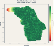
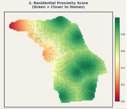
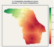
For every square, I measured the straight-line distance from its center point to the nearest road, the nearest home, and the nearest competitor shop. Each distance was then turned into a score between 0 and 1, using two simple rules: closer is better for roads and homes, farther is better for competitors.
Click a tab below to switch between the three criteria and see how each one looks on the map.
Step Four — Combining Everything Into One Final Score
Now the three scores get multiplied by their weights and added together. Every square ends up with one final number between 0 and 1, which is then sorted into three simple groups: Low, Medium, and High suitability.

| Suitability Level | Score Range | What It Means |
|---|---|---|
| High | 0.70 – 1.00 | Great access, near homes, away from rivals |
| Medium | 0.40 – 0.70 | Decent, but weak on one or more factors |
| Low | 0.00 – 0.40 | Hard to reach, few nearby customers, or too close to a competitor |
Where This Method Can Go Wrong
All the road, home, and shop data in this project comes from OpenStreetMap, which is built by volunteers. This is powerful and free, but not perfect. A brand-new residential block or a small local shop that nobody has mapped yet simply will not show up in the data, even though it exists in real life.
That is why the whole workflow is built in separate, swappable steps. If a real client gives me their own accurate shapefiles, GPS survey data, or official city planning maps, I can plug that data directly into the same scoring formulas without rewriting the analysis from scratch.
Closing Thoughts
This project turns a question that usually depends on gut feeling — "where should I open my shop?" — into something measurable, repeatable, and visual. The same three-step method (score, weigh, combine) can be reused for almost any location decision: where to build a school, a clinic, a warehouse, or a bus stop.
The full notebook, along with the raw data pipeline, is open for review on my GitHub.